I was assigned a college project on graphs and decided to share my implementation with the world since these are very interesting and useful data structures. Also, I got a great score at it so I guess it should be good enough to go public and to be the blog’s square one.
Below is a picture of the graph in my assignment:
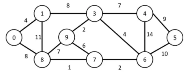
The image shows a graph that is both undirected – since edges (also known as links) such as 8 → 7 are equivalent to 7 → 8 – and weighted, as each edge is assigned a value that typically represents the cost, distance, or strength of the connection between two vertices (or nodes).
Although these data structures are usually pictured like the screenshot above i.e. with clear, rounded vertices and weights, in real life, people work with representations of graphs. To achieve this, two main ways of describing them were developed:
For the remaining of this article, the graph will be treated as an adjacency list.
Code description
In this and in the following sections, I’ll discuss theory and code. You may treat the code snippets
as pseudocode for the sole fact that important NULL
checks are stripped for brevity.
However, the described steps in algorithm sections represent actual procedures in these routines.
The program’s entrypoint, main.c, contains the actual
usage and tests
of the API. The API itself is declared and defined in graph.h and graph.c
respectively.
A queue is also implemented as an
auxiliary data structure for graph traversal.
In graph.h, some data types are created to describe
the graph:
typedef struct _neighbour {
    int vertexValue;
    float weight;
    struct _neighbour*  next;
} Neighbour;

typedef struct _graph {
    int nv;    /* amount of vertices */
    int ne;    /* amount of edges */
    Neighbour** nb; /* nb[i] points to the list of edges that affects i */
} Graph;
The Neighbour struct represents an adjacency list of
an arbitrary vertex i – showing
the vertexValue of the neighbouring node, the weight of its edge and a pointer to the
next possible neighbouring
node of i. You can keep traversing this linked list
until you hit the case in which next is NULL, indicating
that there are no more neighbours of i left.
The Graph type includes two simple integer counters
that track the maximum number of vertices nv
– read-only, passed during initialization – and the number of edges ne that grows as these are
included in the data structure.
The Neighbour** nb field represents the actual
graph as a list of adjacency lists: you get the neighbours of
a given vertex i by reading nb[i] in linear time.
I should say, though, that the graph.h was supplied
as part of the assignment and, thus, I couldn’t really
think of new, interesting ways of representing the graph, but I am sure someone else thought about it:
it’s a whole part of Computer Science.
The last custom type is called Edge which I created
for use in Kruskal’s algorithm:
// Used for Kruskal's algorithm
typedef struct _edge {
    int u, v;
    float weight;
} Edge;
The Edge data type houses all the necessary
information for describing an edge of a graph.
The two vertices u and v along with the weight of the edge
between them are all the information
needed
to generate a minimum spanning tree. More on that later.
The functions exposed by graph.h are listed below:
Graph* create_graph(int nv);
void add_edge(Graph* g, int vertex1, int vertex2, float weight);
void print_as_adjacency_list(Graph* g);
void print_as_adjacency_matrix(Graph* g);
void bfs(Graph* g, int initialVertexValue);
Graph* kruskal(Graph* g);
void free_graph(Graph* g);
I won’t go into all these functions, as many are straightforward and common in C programming.
I'll focus on bfs, kruskal, and some helper functions that will show up later.
Even though it may be considered a simple topic for technical readers, I’ll unfurl the queue implementation for a matter of completion. Feel free to skip it, if you fancy.
In queue.h, two custom types are created:
typedef struct _queueNode {
    Neighbour* nb;
    struct _queueNode* next;
} QueueNode;

typedef struct _queue {
    QueueNode* front;
    QueueNode* back;
} Queue;
The queue will only be used in the breadth-first search algorithm. As such, the QueueNode
type only needs a pointer
to the adjacency list of the current vertex nb and
another one for the next node in queue.
The Queue itself has members for the front and the
back of the ADT, since
constant time will be needed for both front read and
back write – after all, this is where this data
structure excels.
The exposed functions are:
Queue* create_queue();
void enqueue(Queue* Queue, Neighbour* nb);
QueueNode* dequeue(Queue* Queue);
int is_queue_empty(Queue* Queue);
void free_queue(Queue* Queue);
Pretty usual stuff. Both enqueue and dequeue run in O(1) time just like a
standard queue.
is_queue_empty evaluates the q->front pointer giving us information on remaining
vertices in queue.
Consequently, it can – and will – be used to control the graph traversal.
A point that’s worth mentioning is that my dequeue
implementation encompasses both peeking and popping, i.e.
it returns the QueueNode in front of the queue and
moves on with it. I found this approach
straightforward, even though you have to be extra careful regarding leaking
memory and losing information.
Breadth-first search (BFS)
The BFS implementation (bfs in
graph.c)
starts with the creation of two auxiliary structures necessary for the graph traversal logic.
A verticesToVisit queue which holds enqueued vertices
during the traversal for the later exploration
of their neighbours.
/*
Performs breadth-first search (BFS)
*/
void bfs(Graph* g, int initialVertexValue) {
    if (!g) return;

    // Queue and visited vertices list creation
    Queue* verticesToVisit = create_queue();

    int* visited = (int*) calloc(g->nv, sizeof(int));
The visited array is a pointer of int and is allocated using calloc.
Unlike malloc, the college canon,
this function allocates a block of memory and zero
initializes all of its bytes to zero.
Due to this behavior, I could leverage the initial status of zero (false) in the visited array as a
way of saying that all
vertices were initially unvisited, which makes sense.
At the end of the day, this array is just a pointer to boolean states, so you may query
visited[i] of a given vertex i and check its result: 1 in case it has been
visited,
0 otherwise.
The gist of the BFS algorithm lies in a do {...} while() loop. The old implementation I made used
a while loop, but it
featured an auxiliary, heap allocated variable to be enqueued, making the checked condition evaluate to true,
and, thus, allowing the loop to start.
I do not know if I made the right decision – if there’s such a thing –, but I refactored the code to
leverage the former C construct.
    do {
        QueueNode* qn = dequeue(verticesToVisit);
        int currentVertexValue;
        Neighbour* currentVertexNeighbours;

        if (!qn) {
            // First pass

        } else {
            // Subsequent passes

        }

    } while(!is_queue_empty(verticesToVisit));
It was an interesting refactor because a do {...} while() enters the loop’s body immediately
and evaluates its condition afterwards,
so it’s like the semantics of it express that the initial run will be different (which it is).
It also discarded
the use of the previously mentioned helper variable and hacky first-time enqueuing.
The refactoring did lead to some branching in the loop’s internal (to check if it’s a first run), but I don’t
think it negatively impacted
readability. I know do {...} while() loops aren’t new
in programming, but I rarely used them. Frankly, though, using them in this context
exposed me to a new way of thinking about the problem, which is an integral part of
the engineering
ethos.
Dequeuing from an empty queue will return a NULL
pointer, which means the program is faced with the initial case
of the traversal (first run of the algorithm).
The variable currentVertexValue is assigned to initialVertexValue (vertex chosen by
the user to start BFS
from), and
then used to obtain the adjacency list of it (currentVertexNeighbours).
        if (!qn) {
            // First pass
            currentVertexValue = initialVertexValue;

            printf("Visiting %d\n", currentVertexValue);
            visited[currentVertexValue] = 1;

            currentVertexNeighbours = g->nb[currentVertexValue];

        }
In order for the algorithm to properly work, the initial vertex has to be immediately marked as visited in this branch, otherwise, when it’s found during traversal, it will be revisited.
The else branch will run for subsequent vertices.
Here, the dequeued qn node won’t be NULL and the currentVertex is
extracted from it. Then, currentVertexValue
and currentVertexNeighbours are obtained by reading
the corresponding struct pointers.
        } else {
            // Subsequent passes
            Neighbour* currentVertex = qn->nb;
            currentVertexValue = currentVertex->vertexValue;

            currentVertexNeighbours = g->nb[currentVertexValue];

            free(currentVertex);
            free(qn);
        }
After the branching is done, the actual traversal in the vertice’s adjacency list begins:
        // After acquiring a vertex, iterate through all of its neighbours
        while (currentVertexNeighbours) {
            currentVertexValue = currentVertexNeighbours->vertexValue;
            if (!visited[currentVertexValue]) {
                /*
                If the vertex hasn't been visited yet, visit it
                and enqueue a copy of it to visit its neighbours later on
                */
                printf("Visiting %d\n", currentVertexValue);
                visited[currentVertexValue] = 1;

                Neighbour* vertexCopy = (Neighbour*) malloc(sizeof(Neighbour));

                // allocation check and pointer assignment...
                enqueue(verticesToVisit, vertexCopy);
            }
            // walk through the adjacency list
            currentVertexNeighbours = currentVertexNeighbours->next;
        }
This is pretty much like a linked list traversal so it should run in O(E) where E is the number of
edges in the list.
There’s also a copying step along with the visited
array so the implementation should have O(V) space complexity on average
(where V is the amount of vertices in the graph). In spite of this, the time complexity of the algorithm is
O(V+E) since all vertices and edges are explored.
Starting from vertex 0, the order in which the vertices of the analyzed graph are visited is shown below:
Visiting 0
Visiting 8
Visiting 1
Visiting 7
Visiting 9
Visiting 3
Visiting 6
Visiting 4
Visiting 5
Kruskal's algorithm
The desired outcome from running Kruskal’s
(kruskal in graph.c) is to have a
minimum spanning tree (MST)
at the end of the algorithm. In essence, a MST is a subgraph of an undirected and weighted graph
that connects all vertices without forming any cycles and has the minimum possible total edge weight.
As an example, MSTs can be used in network design for establishing a topology which ensures all elements (vertices) are connected with the least piping cost (minimum total edge weight)! How’s that for engineering the Internet?

Partial map of Internet in 2005 by the OPTE project
Image extracted from Wikipedia and subject to Creative Commons
Kruskal is a greedy algorithm, and as such, works
heuristically by picking
the immediate best local solution. What that means is that, for this particular case, the graph edges
will be sorted by ascending weights,
and then, the ones with the minimal weight that connect two vertices and do not form a cycle are immediately
added to the tree,
without ever considering if, in the grand scheme of things, this arrangement will be global optimal
solution.
Given the relatively sparse graph in this assignment, the locally optimal solution should be sufficiently close to the global one. After all, there are only 14 edges, so the approximation, if any, should be a fair trade.
In case my explanation of greedy algorithms was too fleeting, I’ll leave a helpful analogy that I came across in the article 40 Key Computer Science Concepts Explained In Layman’s Terms:
Imagine you are going for hiking and your goal is to reach the highest peak possible. You already have the map before you start, but there are thousands of possible paths shown on the map. You are too lazy and simply don’t have the time to evaluate each of them. Screw the map! You started hiking with a simple strategy – be greedy and short-sighted. Just take paths that slope upwards the most.
After the trip ended and your whole body is sore and tired, you look at the hiking map for the first time. Oh my god! There’s a muddy river that I should’ve crossed, instead of keep walking upwards.
A greedy algorithm picks the best immediate choice and never reconsiders its choices.
Past the theoretical discussion, let us get our hands dirty in the implementation:
/*
Returns the minimum spanning tree
(subgraph that contains all vertices and doesn't have cycles)
*/
Graph* kruskal(Graph* g) {
    if (!g) return NULL;

    // Firstly, store all edges
    Edge* edges = (Edge*) malloc(g->ne * sizeof(Edge));

    .......
}
A block of memory is allocated for all inserted edges in the graph. This isn’t great since there’s a chance that not each and every edge will be analyzed. I’ll explain that in detail later, but for now, let’s assume all of them will be used.
Next, the entirety of the graph is traversed in its V vertices and E edges using the adjacency lists.
So this nested for
loop runs in O(V+E) linear time.
    int edgeIndex = 0;
    for (int i = 0; i < g->nv; i++) {
        for (Neighbour* nb = g->nb[i]; nb != NULL; nb = nb->next) {
            // Perform deduplication
            if (i < nb->vertexValue) {
                edges[edgeIndex++] = (Edge) {i, nb->vertexValue, nb->weight};
            }
        }
    }
An if clause is responsible for storing and deduplicating edges as the
graph is undirected. The conditional only stores edges (u, v) where u < v. This is a design matter, since
picking
the edge when u is greater will also achieve deduplication, but I think that selecting the edges in ascending
order is somehow more intuitive.
Once the edges are collected, they have to be sorted. I used the C library qsort, which,
despite its name is not guaranteed be quicksort.
    // Sort the edges by weight
    qsort(edges, g->ne, sizeof(Edge), _compare_edges);
At this point, one of the helper functions I mentioned earlier shows itself:
// Compares two edges by their weight
static int _compare_edges(const void* a, const void* b) {
    Edge* edgeA = (Edge*) a;
    Edge* edgeB = (Edge*) b;
    if (edgeA->weight < edgeB->weight) return -1;
    if (edgeA->weight > edgeB->weight) return 1;
    return 0;
}
The argument types and return branches are determined by qsort’s API. I just made the function
comply to it.
Up next, two crucial heap allocated structures are created. The first one is called parents
and is
responsible
for creating a forest consisting of single node trees for every vertex in the graph.
    // Initialize the Union-Find DS
    int* parents = (int*) malloc(g->nv * sizeof(int));
    int* rank = (int*) calloc(g->nv, sizeof(int));

    // Initially, each vertex is the parent of the set that contains itself
    for (int i = 0; i < g->nv; i++) {
        parents[i] = i;
    }
The rank array is a heuristic approach to each tree’s
height. Since it’s calloc allocated, all
trees initially have rank 0. It will be used for updating the forest as the vertices are connected in
Kruskal’s
main loop. These two variables make up a Union-Find data structure.
Finally, we get to the core of the matter: the for
loop.
    // Initializes the minimum spanning tree (MST)
    Graph* mst = create_graph(g->nv);

    /*
    Kruskal's main loop:
    the loop continues until all edges are included in the MST
    OR the MST is complete, that is, it has g->nv - 1 edges
    The edges are processed in ascending order, due to previous sorting
    */
    for (int i = 0, includedEdges = 0; i < g->ne && includedEdges < g->nv - 1; i++) {
Notice how the minimum spanning tree is of type Graph*. This not only makes the implementation
simpler by
reducing the quantity of custom types, but makes perfect sense since trees are special cases of
graphs.
The block comment above the loop should make the condition checking logic clear, but I’ll add a note
on the loop initialized variables. In the one hand, the variable i
indexes the edges array, providing access to the
struct pointers u, v, and weight. It is also
used for bounds checking (i < g->ne) preventing
invalid memory access, and for
halting the algorithm after all edges are checked.
On the other hand, the includedEdges variable keeps
track of inserted edges and stops the algorithm once it’s equal to
g->nv - 1: the
spanning tree of a
given
graph with V vertices is complete once it has V - 1 edges.
Inside the loop, all information regarding the currently analyzed edge i is accessed:
        int u = edges[i].u;
        int v = edges[i].v;
        float weight = edges[i].weight;
For the next step, a conditional statement safeguards the crux of Kruskal’s: adding the edge of two vertices without forming cycles in the tree.
        /*
        If this conditional statement is true, it's safe to add the edge to the MST.
        Since they have different parents, they are in disjoint sets (different trees).
        Thus, no cycle will be formed
        */
        if (_find(parents, u) != _find(parents, v)) {
If the vertex already is the root of the tree (parent of the set) containing itself, the _find
function returns
its value immediately. This scenario should be more common at the start of the routine, when each vertex is
in
its
own tree.
// Search with path compression, avoiding cycles in the MST
static int _find(int* parents, int vertex) {
    if (parents[vertex] != vertex) {
        // Compression ("flattens" the tree): as the call stack unwinds, previous vertices point to the parent of the set
        parents[vertex] = _find(parents, parents[vertex]);
    }

    // Vertex already is the root/parent of current set
    return parents[vertex];
}
Otherwise, it leverages recursion to find the parent of a given vertex already included in the incipient MST. Here, something amazing happens: until the base case is reached, all the vertices deep in recursion will have their parent’s value assigned to the value returned by the function calls.
This optimization is called path
compression
and makes paths to the set’s parent shorter, quickening subsequent _find calls.
Human ingenuity is amazing!
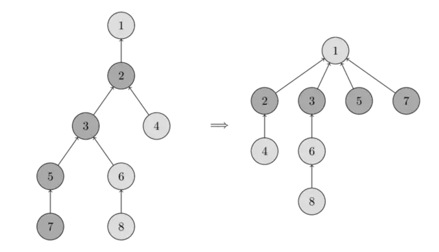 Image extracted from Algorithms for Competitive
Programming.
Image extracted from Algorithms for Competitive
Programming.
Notice how the tree on the right is flatter.
After _find is called for the first time, checking
whether two vertices u and v are in the same set
should be faster as the set’s representative will probably be read in O(1). Unless the graph is too
dense,
the entirety of nodes won’t be traversed for the parent check.
In case u and v are NOT in the same set, the conditional evaluates to true:
if (_find(parents, u) != _find(parents, v)) {
and they can be included in the MST:
add_edge(mst, u, v, weight);
As the vertices are now in the same set (the MST), the Union Find structure has to be updated:
            // Joins the sets of both vertices to reflect the current nature of the MST post edge inclusion
            _unionSets(parents, rank, u, v);
            includedEdges++;
The _unionSets function does u ∪ v, taking the
ranks of both trees in account:
// Performs union (U) of two, initially disjoint, sets
static void _unionSets(int* parents, int* rank, int u, int v) {
    int rootU = _find(parents, u);
    int rootV = _find(parents, v);

    // Picks the set with greatest rank as the representative
    if (rootU != rootV) {
        if (rank[rootU] > rank[rootV]) {
            parents[rootV] = rootU;
        } else if (rank[rootU] < rank[rootV]) {
            parents[rootU] = rootV;
        } else {
            parents[rootV] = rootU;
            rank[rootU]++;
        }
    }
}
Inside the if clause lies the mechanism by which two sets are joined. The set with the greatest rank – recall that it’s a heuristic for a tree’s height – is selected as the root of the new u ∪ v set. This ensures that the tree doesn’t grow unnecessarily since the smaller tree’s rank won’t affect the larger one’s.
In case both sets have the same rank, the first one (u) is arbitrarily picked as the representative of the new set and its rank is incremented by one.
Sorting dominates the runtime of Kruskal’s algorithm so the main loop shouldn’t affect runtime as much as the former step.
Once the algorithm is done, auxiliary data structures are freed and the MST is returned to the caller:
    free(edges);
    free(parents);
    free(rank);

    return mst;
Usage example
Now that some properties and algorithms of graphs were explained, I’ll put our discussion in practice
by analyzing main.c. I made the assignment using a TDDish
perspective, so I’ll first list what the binary is expected to achieve, and later show its source.
- Create the graph itself (as we’ve seen, a representation of it)
- Add the edges that make up the graph in the assignment
- Pretty print the graph to
stdoutas an adjacency list and as an adjacency matrix - Print the visited vertices in BFS order starting from vertex 0
- Using Kruskal’s algorithm, obtain a minimum spanning tree (MST)
- Pretty print the MST to
stdoutas an adjacency list and as an adjacency matrix - Correctly manage memory while doing all of that (so no segfaults, leaks, etc)
Most of these are clearly addressed in the binaries entrypoint (main.c):
#include <stdio.h>
#include <assert.h>
#include "graph.h"

// Maximum number of vertices
#define MAX_GRAPH_SIZE 30

int main() {
    Graph* g = create_graph(MAX_GRAPH_SIZE);
    if (!g) {
        return -1;
    }

    // 14 edges in the graph
    add_edge(g, 0, 1, 4.0);
    add_edge(g, 0, 8, 8.0);
    add_edge(g, 8, 1, 11.0);
    add_edge(g, 3, 1, 8.0);
    add_edge(g, 3, 9, 2.0);
    add_edge(g, 9, 8, 7.0);
    add_edge(g, 7, 8, 1.0);
    add_edge(g, 7, 9, 6.0);
    add_edge(g, 4, 3, 7.0);
    add_edge(g, 3, 6, 4.0);
    add_edge(g, 4, 6, 14.0);
    add_edge(g, 4, 5, 9.0);
    add_edge(g, 5, 6, 10.0);
    add_edge(g, 6, 7, 2.0);
    assert(g->ne == 14);

    printf("Graph as adjacency list:\n");
    print_as_adjacency_list(g);

    printf("Graph as adjacency matrix:\n");
    print_as_adjacency_matrix(g);

    printf("\n");
    bfs(g, 0);

    Graph* mst = kruskal(g);
    if (!mst) {
        return -1;
    }

    printf("Spanning tree as adjacency list:\n");
    print_as_adjacency_list(mst);

    printf("\nSpanning tree as adjacency matrix:\n");
    print_as_adjacency_matrix(mst);

    free_graph(mst);
    free_graph(g);

    return 0;
}
Since all the 14 edges have to be inserted, I used an assert call there.
Don’t do this for production code though, as this, under
usual circumstances, abnormally terminates your program.
To ensure that memory management is correct, I used Valgrind:
gcc -g -Wall -Wextra main.c graph.c queue.c -o graphs
valgrind -s --track-origins=yes --leak-check=full ./graphs
Thankfully, its output indeed shows no errors or leaks:
HEAP SUMMARY:
    in use at exit: 0 bytes in 0 blocks
  total heap usage: 132 allocs, 132 frees, 10,720 bytes allocated

All heap blocks were freed -- no leaks are possible

ERROR SUMMARY: 0 errors from 0 contexts (suppressed: 0 from 0)
The program’s standard output:
./graphs
Graph as adjacency list:
0: -> 8 (weight: 8.00) -> 1 (weight: 4.00)
1: -> 3 (weight: 8.00) -> 8 (weight: 11.00) -> 0 (weight: 4.00)
3: -> 6 (weight: 4.00) -> 4 (weight: 7.00) -> 9 (weight: 2.00) -> 1 (weight: 8.00)
4: -> 5 (weight: 9.00) -> 6 (weight: 14.00) -> 3 (weight: 7.00)
5: -> 6 (weight: 10.00) -> 4 (weight: 9.00)
6: -> 7 (weight: 2.00) -> 5 (weight: 10.00) -> 4 (weight: 14.00) -> 3 (weight: 4.00)
7: -> 6 (weight: 2.00) -> 9 (weight: 6.00) -> 8 (weight: 1.00)
8: -> 7 (weight: 1.00) -> 9 (weight: 7.00) -> 1 (weight: 11.00) -> 0 (weight: 8.00)
9: -> 7 (weight: 6.00) -> 8 (weight: 7.00) -> 3 (weight: 2.00)
Graph as adjacency matrix:
        0     1     3     4     5     6     7     8     9
  0     0  4.00     0     0     0     0     0  8.00     0
  1  4.00     0  8.00     0     0     0     0 11.00     0
  3     0  8.00     0  7.00     0  4.00     0     0  2.00
  4     0     0  7.00     0  9.00 14.00     0     0     0
  5     0     0     0  9.00     0 10.00     0     0     0
  6     0     0  4.00 14.00 10.00     0  2.00     0     0
  7     0     0     0     0     0  2.00     0  1.00  6.00
  8  8.00 11.00     0     0     0     0  1.00     0  7.00
  9     0     0  2.00     0     0     0  6.00  7.00     0

Visiting 0
Visiting 8
Visiting 1
Visiting 7
Visiting 9
Visiting 3
Visiting 6
Visiting 4
Visiting 5
Spanning tree as adjacency list:
0: -> 8 (weight: 8.00) -> 1 (weight: 4.00)
1: -> 0 (weight: 4.00)
3: -> 4 (weight: 7.00) -> 6 (weight: 4.00) -> 9 (weight: 2.00)
4: -> 5 (weight: 9.00) -> 3 (weight: 7.00)
5: -> 4 (weight: 9.00)
6: -> 3 (weight: 4.00) -> 7 (weight: 2.00)
7: -> 6 (weight: 2.00) -> 8 (weight: 1.00)
8: -> 0 (weight: 8.00) -> 7 (weight: 1.00)
9: -> 3 (weight: 2.00)

Spanning tree as adjacency matrix:
        0     1     3     4     5     6     7     8     9
  0     0  4.00     0     0     0     0     0  8.00     0
  1  4.00     0     0     0     0     0     0     0     0
  3     0     0     0  7.00     0  4.00     0     0  2.00
  4     0     0  7.00     0  9.00     0     0     0     0
  5     0     0     0  9.00     0     0     0     0     0
  6     0     0  4.00     0     0     0  2.00     0     0
  7     0     0     0     0     0  2.00     0  1.00     0
  8  8.00     0     0     0     0     0  1.00     0     0
  9     0     0  2.00     0     0     0     0     0     0
Wrapping up
First of all, if you reached this far I could somehow have your attention for a few minutes, so thank you!
I ran time and perf several times and reviewed the code thoroughly and
can tell that
this project isn’t perfect. There are
lots of potential improvements such as minimizing
system/kernel time by better placing allocations and releases, using memory pools etc.
Refactoring the code for higher testability and cohesion is an
interesting challenge as well. Nonetheless, I must draw the line somewhere.
Originally, the purpose of this post was to reinforce my inkling of experience on graphs and disjoint sets, as my memory can get brittle over time. However, as I wrote it, I realized it can commence a fruitful, long-lasting blogging journey (hopefully). Sharing knowledge with other people and the world matters a lot to me. So, if this reading added value for you, please let me know.
This wasn’t supposed to teach you everything on graphs, disjoint sets, and Kruskal’s. Rather, I hope I made your brain scratch a little with the stuff I narrated.